In this chapter, we examine firm behavior in more detail. This topic will give you a better understanding of the decisions behind the supply curve. In addition, it will introduce you to a part of economics called industrial organization — the study of how firms’ decisions about prices and quantities depend on the market conditions they face.
WHAT ARE COSTS?
We begin our discussion of costs at a Cookie factory. By examining some of the issues that the owner faces in his/her business, we can learn some lessons about costs that apply to all firms in an economy.
Total Revenue, Total Cost, and Profit
The amount that the firm receives for the sale of its output is called its total revenue. The amount that the firm pays to buy inputs is called its total cost. Profit is a firm’s total revenue minus its total cost:
\[ \text{Profit} = \text{Total revenue} - \text{Total cost} \]
To see how a firm goes about maximizing profit, we must consider fully how to measure its total revenue and its total cost. Total revenue is the easy part: It equals the quantity of output the firm produces times the price at which it sells its output. By contrast, the measurement of a firm’s total cost is more subtle.
Costs As Opportunity Costs
explicit costs: input costs that require an outlay of money by the firm implicit costs: input costs that do not require an outlay of money by the firm
Imagine that the owner of the cookie factory is skilled with computers and could earn ¥100 per hour working as a programmer. For every hour that she works at her cookie factory, she gives up ¥100 in income, and this forgone income is also part of her costs. The total cost of her business is the sum of the explicit costs and the implicit costs.
The Cost of Capital as An Opportunity Cost
An important implicit cost of almost every business is the opportunity cost of the financial capital that has been invested in the business. Suppose, for instance, that the owner of the cookie factory used ¥300,000 of her savings to buy her cookie factory from its previous owner. If she had instead left this money deposited in a savings account that pays an interest rate of 5 percent, she would have earned ¥15,000 per year. To own her cookie factory, therefore, Caroline has given up ¥15,000 a year in interest income. This forgone ¥15,000 is one of the implicit opportunity costs of Caroline’s business.
Economic Profit Versus Accounting Profit
Now let’s return to the firm’s objective: profit. An economist measures a firm’s economic profit as the firm’s total revenue minus all the opportunity costs (explicit and implicit) of producing the goods and services sold. An accountant measures the firm’s accounting profit as the firm’s total revenue minus only the firm’s explicit costs as shown in Figure 1.
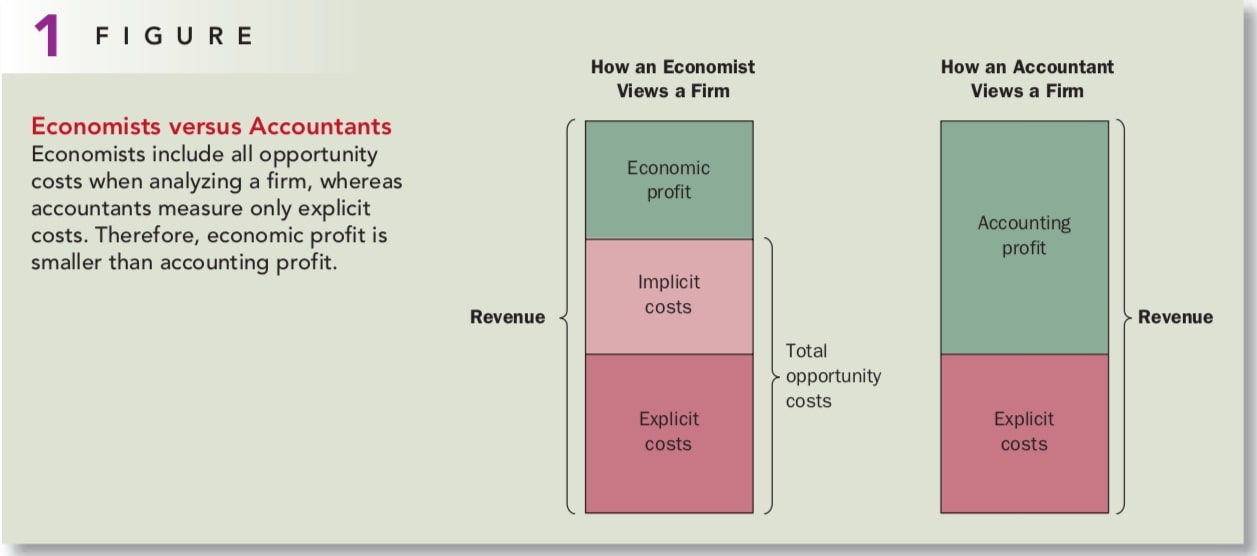
Economic profit is an important concept because it is what motivates the firms that supply goods and services. As we will see, a firm making positive economic profit will stay in business. It is covering all its opportunity costs and has some revenue left to reward the firm owners. When a firm is making economic losses, the business owners are failing to earn enough revenue to cover all the costs of production. Unless conditions change, the firm owners will eventually close down the business and exit the industry. To understand business decisions, we need to keep an eye on economic profit.
Economic profit equals to zero means your business is running well and you pay yourself the same amount as you get paid somewhere else.
PRODUCTION AND COSTS
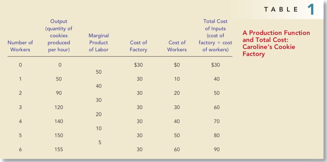
Table 1 shows how the quantity of cookies produced per hour at the cookie factory depends on the number of workers. This relationship between the quantity of inputs (workers) and quantity of output (cookies) is called the production function.
To take a step toward understanding these decisions, the third column in the table gives the marginal product of a worker. Notice that as the number of workers increases, the marginal product declines. The second worker has a marginal product of 40 cookies, the third worker has a marginal product of 30 cookies, and the fourth worker has a marginal product of 20 cookies. This property is called diminishing marginal product.
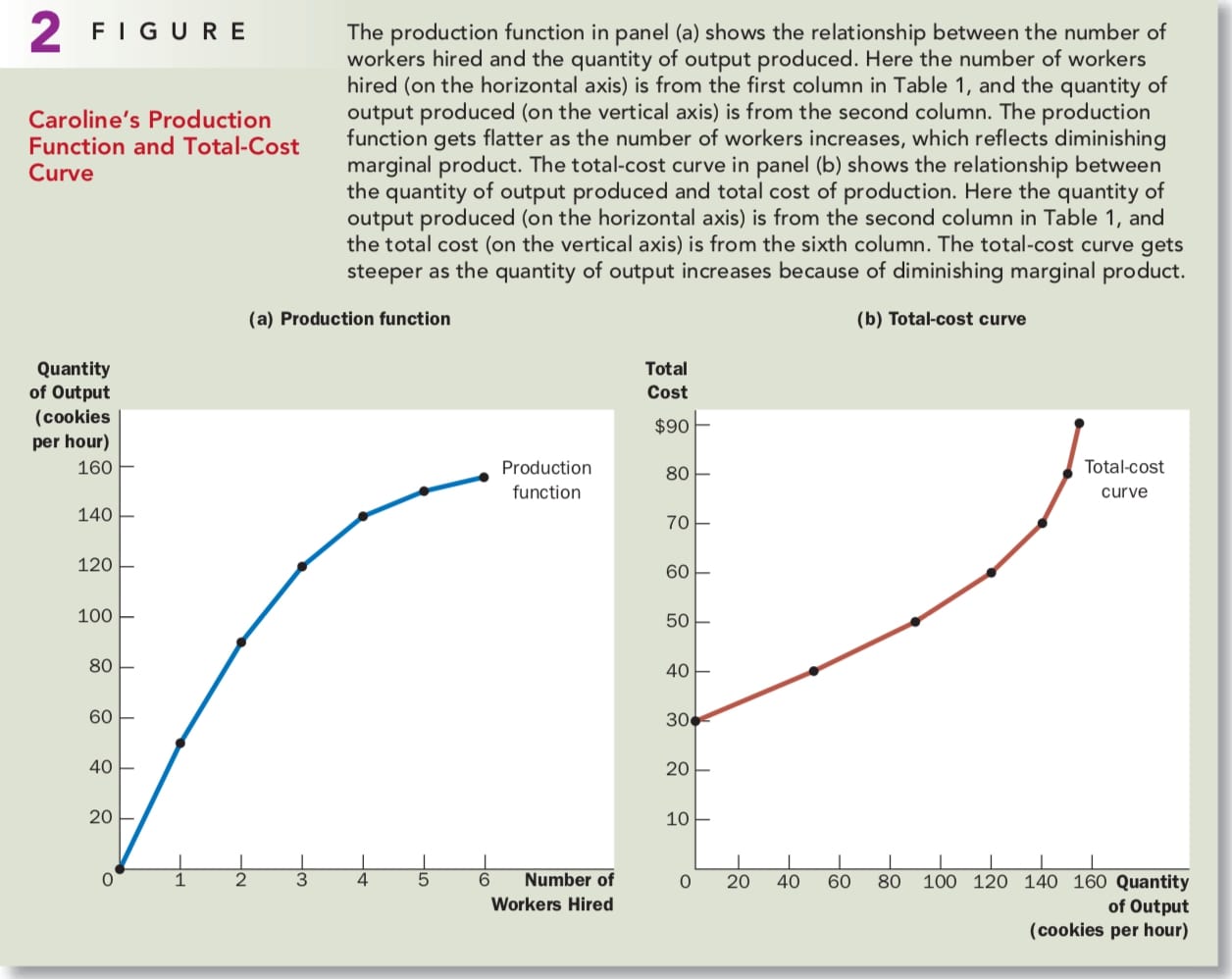
Diminishing marginal product is also apparent in Figure 2. The production function’s slope tells us the change in the factory’s output of cookies for each additional input of labor. That is, the slope of the production function measures the marginal product of a worker. As the number of workers increases, the marginal product declines, and the production function becomes flatter.
From The Production Function To The Total-Cost Curve
Our goal in the next is to study firms’ production and pricing decisions. For this purpose, the most important relationship in Table 1 is between quantity produced and total costs. Panel (b) of Figure 2 graphs these two columns of data with the quantity produced on the horizontal axis and total cost on the vertical axis. This graph is called the total-cost curve.
Now compare the total-cost curve in panel (b) with the production function in panel (a). These two curves are opposite sides of the same coin. The total-cost curve gets steeper as the amount produced rises, whereas the production function gets flatter as production rises. These changes in slope occur for the same reason. High production of cookies means that Caroline’s kitchen is crowded with many workers. Because the kitchen is crowded, each additional worker adds less to production, reflecting diminishing marginal product. Therefore, the production function is relatively flat. But now turn this logic around: When the kitchen is crowded, producing an additional cookie requires a lot of additional labor and is thus very costly. Therefore, when the quantity produced is large, the total-cost curve is relatively steep.
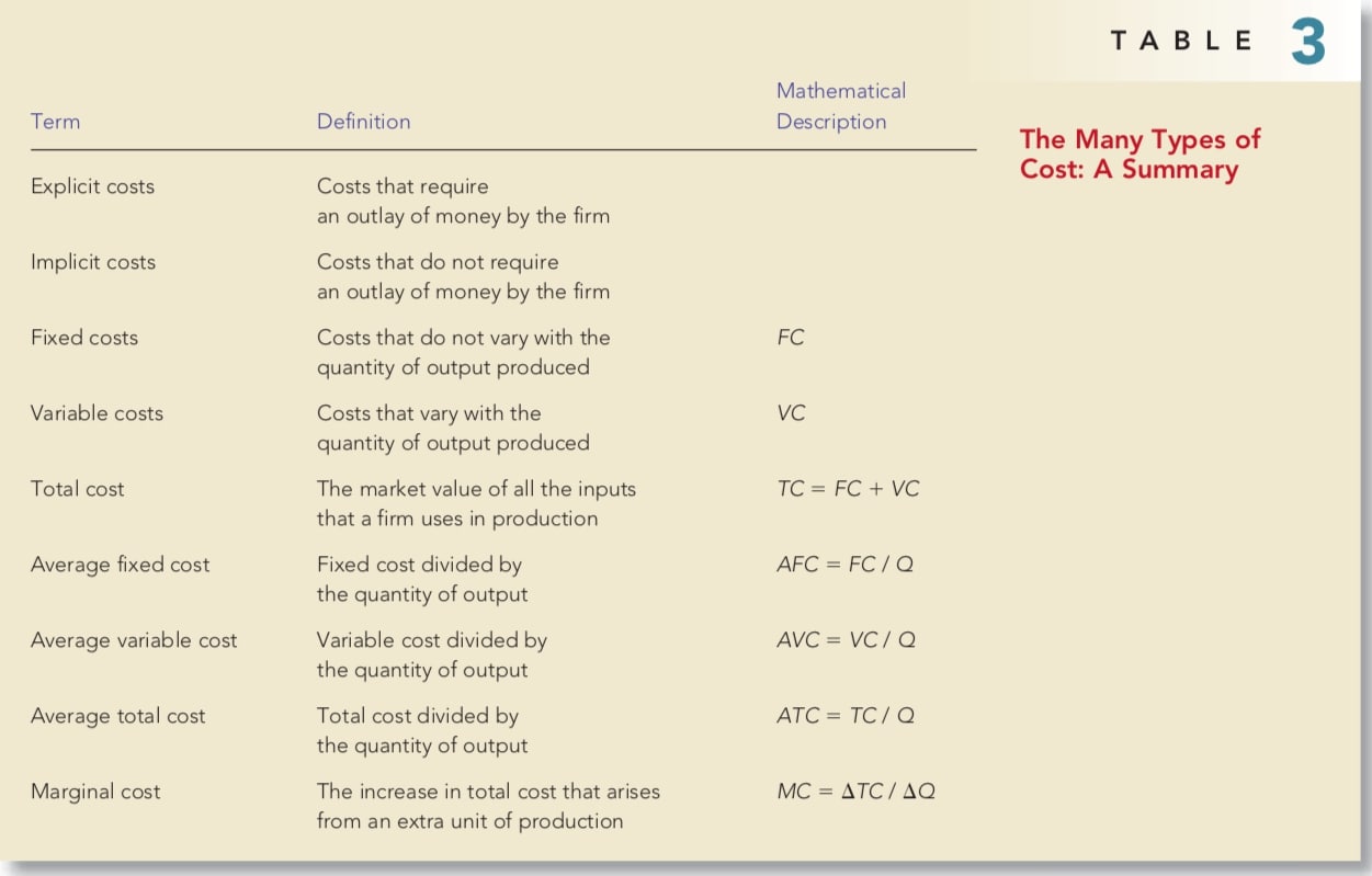
THE VARIOUS MEASURES OF COST
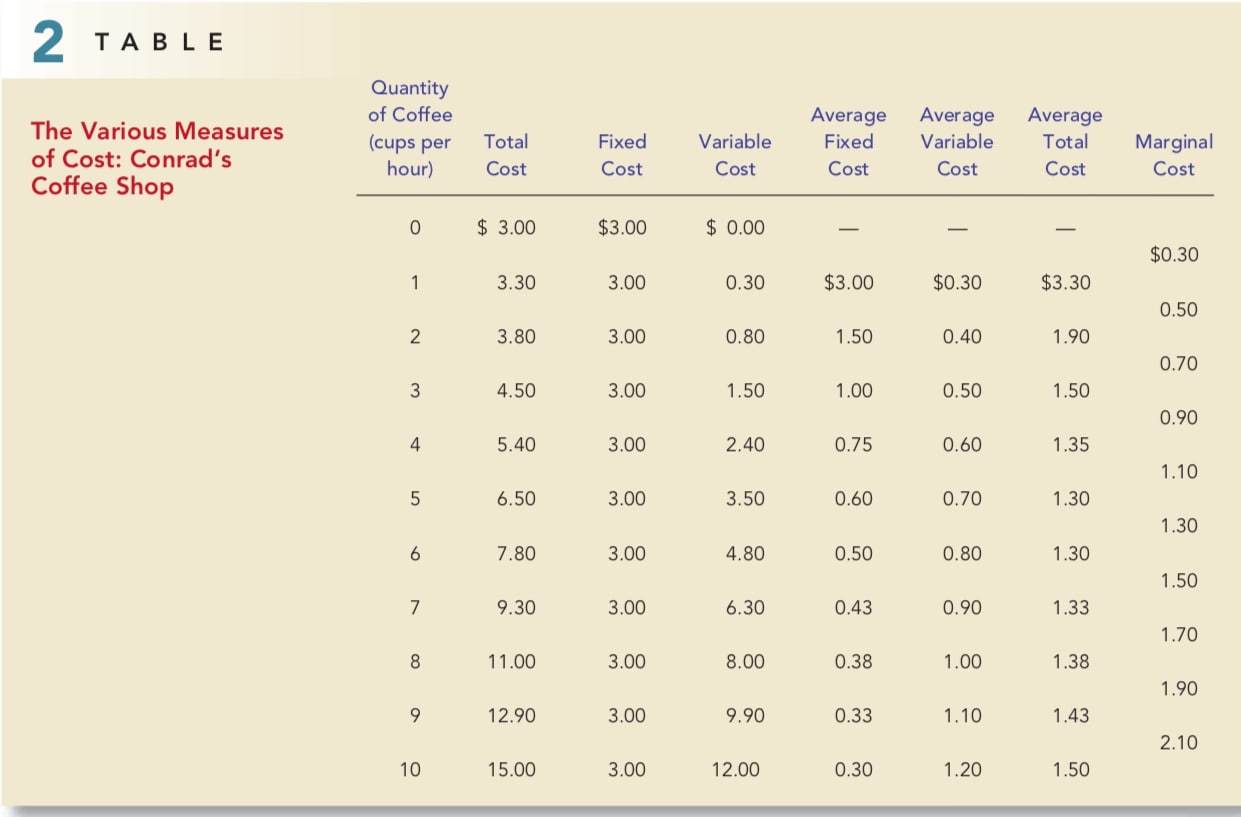
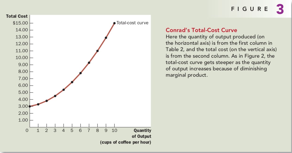
To see how related measures of cost are derived, we consider the example in Table 2. This table presents cost data on Conrad’s Coffee Shop. Figure 3 plots Conrad’s total-cost curve. Conrad’s total-cost curve becomes steeper as the quantity produced rises, which (as we have discussed) reflects diminishing marginal product.
Fixed And Variable Costs
Fixed costs are costs that do not vary with the quantity of output produced. They are incurred even if the firm produces nothing at all. Conrad’s fixed costs include any rent he pays because this cost is the same regardless of how much coffee he produces.
Variable costs are costs that change as the firm alters the quantity of output produced. Conrad’s variable costs include the cost of coffee beans, milk, sugar, and paper cups: The more cups of coffee Conrad makes, the more of these items he needs to buy.
A firm’s total cost is the sum of fixed and variable costs. In Table 2, total cost in the second column equals fixed cost in the third column plus variable cost in the fourth column.
Average and Marginal Cost
Total cost divided by the quantity of output is called average total cost. Because total cost is the sum of fixed and variable costs, average total cost can be expressed as the sum of average fixed cost and average variable cost. Average fixed cost is the fixed cost divided by the quantity of output, and average variable cost is the variable cost divided by the quantity of output.
Although average total cost tells us the cost of the typical unit, it does not tell us how much total cost will change as the firm alters its level of production. Marginal cost is the increase in total cost that arises from an extra unit of production. In the table, the marginal cost appears halfway between two rows because it represents the change in total cost as quantity of output increases from one level to another.
Mathematically:
\[ ATC = TC/Q \\ MC = \triangle TC / \triangle Q \]
Cost Curves And Their Shapes
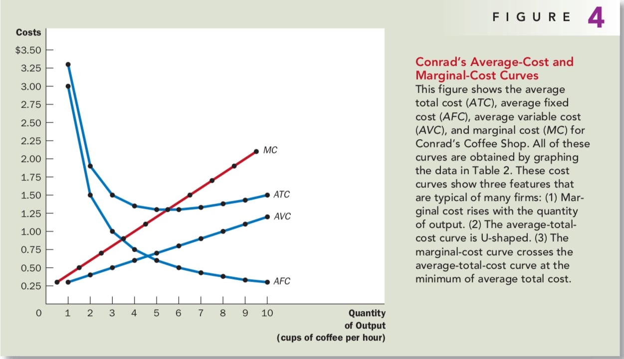
Figure 4 graphs Conrad’s costs using the data from Table 2. The horizontal axis measures the quantity the firm produces, and the vertical axis measures marginal and average costs. The graph shows four curves: average total cost (ATC), average fixed cost (AFC), average variable cost (AVC), and marginal cost (MC).
Rising Marginal Cost Conrad’s marginal cost rises with the quantity of out- put produced. This reflects the property of diminishing marginal product.
U-Shaped Average Total Cost Average total cost is the sum of average fixed cost and average variable cost. Average fixed cost always declines as output rises because the fixed cost is spread over a larger number of units. Average variable cost typically rises as output increases because of diminishing marginal product. Average total cost reflects the shapes of both average fixed cost and average variable cost.
The bottom of the U-shape occurs at the quantity that minimizes average total cost. This quantity is sometimes called the efficient scale of the firm. At the efficient scale, these two forces are balanced to yield the lowest average total cost.
The Relationship Between Marginal Cost and Average Total Cost * Whenever marginal cost is less than average total cost, average total cost is falling. * Whenever marginal cost is greater than average total cost, average total cost is rising.
To see why, consider an analogy. Average total cost is like your cumulative grade point average. Marginal cost is like the grade in the next course you will take. If your grade in your next course is less than your grade point average, your grade point average will fall. If your grade in your next course is higher than your grade point average, your grade point average will rise. The mathematics of average and marginal costs is exactly the same as the mathematics of average and marginal grades.
This relationship between average total cost and marginal cost has an important corollary: The marginal-cost curve crosses the average-total-cost curve at its minimum. As you will see in the next chapter, minimum average total cost plays a key role in the analysis of competitive firms.
Typical Cost Curves
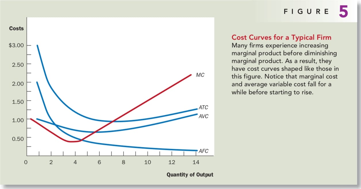
Actual firms are usually more complicated than what we talked about before. In many firms, marginal product does not start to fall immediately after the first worker is hired. Depending on the production process, the second or third worker might have a higher marginal product than the first because a team of workers can divide tasks and work more productively than a single worker. Firms exhibiting this pattern would experience increasing marginal product for a while before diminishing marginal product set in.
Figure 5 shows the cost curves for such a firm, including average total cost (ATC), average fixed cost (AFC), average variable cost (AVC), and marginal cost (MC). Despite these differences from our previous example, the cost curves shown here share the three properties that are most important to remember:
- Marginal cost eventually rises with the quantity of output.
- The average-total-cost curve is U-shaped.
- The marginal-cost curve crosses the average-total-cost curve at the minimum of average total cost.
CONCLUSION